10 minutes to xorbits.pandas#
This is a short introduction to xorbits.pandas which is originated from pandas’ quickstart.
Customarily, we import and init as follows:
In [1]: import xorbits

In [2]: import xorbits.numpy as np

In [3]: import xorbits.pandas as pd

In [4]: xorbits.init()
Object creation#
Creating a Series by passing a list of values, letting it create a default integer index:
In [5]: s = pd.Series([1, 3, 5, np.nan, 6, 8])

In [6]: s
Out[6]:
0    1.0
1    3.0
2    5.0
3    NaN
4    6.0
5    8.0
dtype: float64
Creating a DataFrame by passing an array, with a datetime index and labeled columns:
In [7]: dates = pd.date_range('20130101', periods=6)

In [8]: dates
Out[8]:
DatetimeIndex(['2013-01-01', '2013-01-02', '2013-01-03', '2013-01-04',
               '2013-01-05', '2013-01-06'],
              dtype='datetime64[ns]', freq='D')

In [9]: df = pd.DataFrame(np.random.randn(6, 4), index=dates, columns=list('ABCD'))

In [10]: df
Out[10]:
                   A         B         C         D
2013-01-01 -0.540123  1.188216  0.272509 -1.837075
2013-01-02  0.215270 -1.585255  0.150988 -0.169847
2013-01-03 -2.133070 -1.139072  0.072212  1.876281
2013-01-04  0.930500  0.972882  1.250644 -0.625353
2013-01-05  0.035330  1.419835  0.972366  0.008734
2013-01-06  0.397681  1.916288 -0.970264 -2.139933
Creating a DataFrame by passing a dict of objects that can be converted to series-like.
In [11]: df2 = pd.DataFrame({'A': 1.,
   ....:                     'B': pd.Timestamp('20130102'),
   ....:                     'C': pd.Series(1, index=list(range(4)), dtype='float32'),
   ....:                     'D': np.array([3] * 4, dtype='int32'),
   ....:                     'E': 'foo'})
   ....:

In [12]: df2
Out[12]:
     A          B    C  D    E
0  1.0 2013-01-02  1.0  3  foo
1  1.0 2013-01-02  1.0  3  foo
2  1.0 2013-01-02  1.0  3  foo
3  1.0 2013-01-02  1.0  3  foo
The columns of the resulting DataFrame have different dtypes.
In [13]: df2.dtypes
Out[13]:
A           float64
B    datetime64[ns]
C           float32
D             int32
E            object
dtype: object
Viewing data#
Here is how to view the top and bottom rows of the frame:
In [14]: df.head()
Out[14]:
                   A         B         C         D
2013-01-01 -0.540123  1.188216  0.272509 -1.837075
2013-01-02  0.215270 -1.585255  0.150988 -0.169847
2013-01-03 -2.133070 -1.139072  0.072212  1.876281
2013-01-04  0.930500  0.972882  1.250644 -0.625353
2013-01-05  0.035330  1.419835  0.972366  0.008734

In [15]: df.tail(3)
Out[15]:
                   A         B         C         D
2013-01-04  0.930500  0.972882  1.250644 -0.625353
2013-01-05  0.035330  1.419835  0.972366  0.008734
2013-01-06  0.397681  1.916288 -0.970264 -2.139933
Display the index, columns:
In [16]: df.index
Out[16]:
DatetimeIndex(['2013-01-01', '2013-01-02', '2013-01-03', '2013-01-04',
               '2013-01-05', '2013-01-06'],
              dtype='datetime64[ns]', freq='D')

In [17]: df.columns
Out[17]: Index(['A', 'B', 'C', 'D'], dtype='object')
DataFrame.to_numpy() gives a ndarray representation of the underlying data. Note that this
can be an expensive operation when your DataFrame has columns with different data types,
which comes down to a fundamental difference between DataFrame and ndarray: ndarrays have one
dtype for the entire ndarray, while DataFrames have one dtype per column. When you call
DataFrame.to_numpy(), xorbits.pandas will find the ndarray dtype that can hold all
of the dtypes in the DataFrame. This may end up being object, which requires casting every
value to a Python object.
For df, our DataFrame of all floating-point values,
DataFrame.to_numpy() is fast and doesn’t require copying data.
In [18]: df.to_numpy()
Out[18]:
array([[-0.5401225 ,  1.18821624,  0.27250899, -1.83707451],
       [ 0.21527031, -1.58525509,  0.15098758, -0.16984726],
       [-2.1330695 , -1.13907157,  0.07221223,  1.87628112],
       [ 0.93050031,  0.97288153,  1.25064363, -0.62535278],
       [ 0.03532985,  1.41983491,  0.97236569,  0.00873386],
       [ 0.39768145,  1.91628808, -0.9702637 , -2.13993251]])
For df2, the DataFrame with multiple dtypes, DataFrame.to_numpy() is relatively
expensive.
In [19]: df2.to_numpy()
Out[19]:
array([[1.0, Timestamp('2013-01-02 00:00:00'), 1.0, 3, 'foo'],
       [1.0, Timestamp('2013-01-02 00:00:00'), 1.0, 3, 'foo'],
       [1.0, Timestamp('2013-01-02 00:00:00'), 1.0, 3, 'foo'],
       [1.0, Timestamp('2013-01-02 00:00:00'), 1.0, 3, 'foo']],
      dtype=object)
Note
DataFrame.to_numpy() does not include the index or column
labels in the output.
describe() shows a quick statistic summary of your data:
In [20]: df.describe()
Out[20]:
              A         B         C         D
count  6.000000  6.000000  6.000000  6.000000
mean  -0.182402  0.462149  0.291409 -0.481199
std    1.068987  1.454337  0.780227  1.449501
min   -2.133070 -1.585255 -0.970264 -2.139933
25%   -0.396259 -0.611083  0.091906 -1.534144
50%    0.125300  1.080549  0.211748 -0.397600
75%    0.352079  1.361930  0.797402 -0.035911
max    0.930500  1.916288  1.250644  1.876281
Sorting by an axis:
In [21]: df.sort_index(axis=1, ascending=False)
Out[21]:
                   D         C         B         A
2013-01-01 -1.837075  0.272509  1.188216 -0.540123
2013-01-02 -0.169847  0.150988 -1.585255  0.215270
2013-01-03  1.876281  0.072212 -1.139072 -2.133070
2013-01-04 -0.625353  1.250644  0.972882  0.930500
2013-01-05  0.008734  0.972366  1.419835  0.035330
2013-01-06 -2.139933 -0.970264  1.916288  0.397681
Sorting by values:
In [22]: df.sort_values(by='B')
Out[22]:
                   A         B         C         D
2013-01-02  0.215270 -1.585255  0.150988 -0.169847
2013-01-03 -2.133070 -1.139072  0.072212  1.876281
2013-01-04  0.930500  0.972882  1.250644 -0.625353
2013-01-01 -0.540123  1.188216  0.272509 -1.837075
2013-01-05  0.035330  1.419835  0.972366  0.008734
2013-01-06  0.397681  1.916288 -0.970264 -2.139933
Selection#
Note
While standard Python expressions for selecting and setting are
intuitive and come in handy for interactive work, for production code, we
recommend the optimized xorbits.pandas data access methods, .at, .iat,
.loc and .iloc.
Getting#
Selecting a single column, which yields a Series, equivalent to df.A:
In [23]: df['A']
Out[23]:
2013-01-01   -0.540123
2013-01-02    0.215270
2013-01-03   -2.133070
2013-01-04    0.930500
2013-01-05    0.035330
2013-01-06    0.397681
Freq: D, Name: A, dtype: float64
Selecting via [], which slices the rows.
In [24]: df[0:3]
Out[24]:
                   A         B         C         D
2013-01-01 -0.540123  1.188216  0.272509 -1.837075
2013-01-02  0.215270 -1.585255  0.150988 -0.169847
2013-01-03 -2.133070 -1.139072  0.072212  1.876281

In [25]: df['20130102':'20130104']
Out[25]:
                  A         B         C         D
2013-01-02  0.21527 -1.585255  0.150988 -0.169847
2013-01-03 -2.13307 -1.139072  0.072212  1.876281
2013-01-04  0.93050  0.972882  1.250644 -0.625353
Selection by label#
For getting a cross section using a label:
In [26]: df.loc['20130101']
Out[26]:
A   -0.540123
B    1.188216
C    0.272509
D   -1.837075
Name: 2013-01-01 00:00:00, dtype: float64
Selecting on a multi-axis by label:
In [27]: df.loc[:, ['A', 'B']]
Out[27]:
                   A         B
2013-01-01 -0.540123  1.188216
2013-01-02  0.215270 -1.585255
2013-01-03 -2.133070 -1.139072
2013-01-04  0.930500  0.972882
2013-01-05  0.035330  1.419835
2013-01-06  0.397681  1.916288
Showing label slicing, both endpoints are included:
In [28]: df.loc['20130102':'20130104', ['A', 'B']]
Out[28]:
                  A         B
2013-01-02  0.21527 -1.585255
2013-01-03 -2.13307 -1.139072
2013-01-04  0.93050  0.972882
Reduction in the dimensions of the returned object:
In [29]: df.loc['20130102', ['A', 'B']]
Out[29]:
A    0.215270
B   -1.585255
Name: 2013-01-02 00:00:00, dtype: float64
For getting a scalar value:
In [30]: df.loc['20130101', 'A']
Out[30]: -0.5401225034289786
For getting fast access to a scalar (equivalent to the prior method):
In [31]: df.at['20130101', 'A']
Out[31]: Tensor <op=DataFrameLocGetItem, shape=(), key=ee7e4773b7df388abebb4307f872e3d3_0>
Selection by position#
Select via the position of the passed integers:
In [32]: df.iloc[3]
Out[32]: Series(op=DataFrameIlocGetItem)
By integer slices, acting similar to python:
In [33]: df.iloc[3:5, 0:2]
Out[33]: DataFrame <op=DataFrameIlocGetItem, key=cbd7e67e1ae9963c209b0aed5510ba12_0>
By lists of integer position locations, similar to the python style:
In [34]: df.iloc[[1, 2, 4], [0, 2]]
Out[34]: DataFrame <op=DataFrameIlocGetItem, key=c059362b11a04dae5d63d124384d214c_0>
For slicing rows explicitly:
In [35]: df.iloc[1:3, :]
Out[35]: DataFrame <op=DataFrameIlocGetItem, key=ef98d70502f3386377e53e7d6a9a536a_0>
For slicing columns explicitly:
In [36]: df.iloc[:, 1:3]
Out[36]: DataFrame <op=DataFrameIlocGetItem, key=db7538aaea01873192e336c91dbe1997_0>
For getting a value explicitly:
In [37]: df.iloc[1, 1]
Out[37]: Tensor <op=DataFrameIlocGetItem, shape=(), key=ca2f138cfa4deef2241078f1eb17d30d_0>
For getting fast access to a scalar (equivalent to the prior method):
In [38]: df.iat[1, 1]
Out[38]: Tensor <op=DataFrameIlocGetItem, shape=(), key=ca2f138cfa4deef2241078f1eb17d30d_0>
Boolean indexing#
Using a single column’s values to select data.
In [39]: df[df['A'] > 0]
Out[39]:
                   A         B         C         D
2013-01-02  0.215270 -1.585255  0.150988 -0.169847
2013-01-04  0.930500  0.972882  1.250644 -0.625353
2013-01-05  0.035330  1.419835  0.972366  0.008734
2013-01-06  0.397681  1.916288 -0.970264 -2.139933
Selecting values from a DataFrame where a boolean condition is met.
In [40]: df[df > 0]
Out[40]:
                   A         B         C         D
2013-01-01       NaN  1.188216  0.272509       NaN
2013-01-02  0.215270       NaN  0.150988       NaN
2013-01-03       NaN       NaN  0.072212  1.876281
2013-01-04  0.930500  0.972882  1.250644       NaN
2013-01-05  0.035330  1.419835  0.972366  0.008734
2013-01-06  0.397681  1.916288       NaN       NaN
Operations#
Stats#
Operations in general exclude missing data.
Performing a descriptive statistic:
In [41]: df.mean()
Out[41]:
A   -0.182402
B    0.462149
C    0.291409
D   -0.481199
dtype: float64
Same operation on the other axis:
In [42]: df.mean(1)
Out[42]:
2013-01-01   -0.229118
2013-01-02   -0.347211
2013-01-03   -0.330912
2013-01-04    0.632168
2013-01-05    0.609066
2013-01-06   -0.199057
Freq: D, dtype: float64
Operating with objects that have different dimensionality and need alignment. In addition,
xorbits.pandas automatically broadcasts along the specified dimension.
In [43]: s = pd.Series([1, 3, 5, np.nan, 6, 8], index=dates).shift(2)

In [44]: s
Out[44]:
2013-01-01    NaN
2013-01-02    NaN
2013-01-03    1.0
2013-01-04    3.0
2013-01-05    5.0
2013-01-06    NaN
Freq: D, dtype: float64

In [45]: df.sub(s, axis='index')
Out[45]:
                  A         B         C         D
2013-01-01      NaN       NaN       NaN       NaN
2013-01-02      NaN       NaN       NaN       NaN
2013-01-03 -3.13307 -2.139072 -0.927788  0.876281
2013-01-04 -2.06950 -2.027118 -1.749356 -3.625353
2013-01-05 -4.96467 -3.580165 -4.027634 -4.991266
2013-01-06      NaN       NaN       NaN       NaN
Apply#
Applying functions to the data:
In [46]: df.apply(lambda x: x.max() - x.min())
Out[46]:
A    3.063570
B    3.501543
C    2.220907
D    4.016214
dtype: float64
String Methods#
Series is equipped with a set of string processing methods in the str attribute that make it easy to operate on each element of the array, as in the code snippet below. Note that pattern-matching in str generally uses regular expressions by default (and in some cases always uses them).
In [47]: s = pd.Series(['A', 'B', 'C', 'Aaba', 'Baca', np.nan, 'CABA', 'dog', 'cat'])

In [48]: s.str.lower()
Out[48]:
0       a
1       b
2       c
3    aaba
4    baca
5     NaN
6    caba
7     dog
8     cat
dtype: object
Merge#
Concat#
xorbits.pandas provides various facilities for easily combining together Series and
DataFrame objects with various kinds of set logic for the indexes
and relational algebra functionality in the case of join / merge-type
operations.
Concatenating xorbits.pandas objects together with concat():
In [49]: df = pd.DataFrame(np.random.randn(10, 4))

In [50]: df
Out[50]:
          0         1         2         3
0 -0.784413 -0.449676 -0.041251 -2.561293
1 -0.222866 -0.175106 -0.355334 -0.414543
2  1.904357 -0.148607 -0.434686  0.753796
3 -0.104409 -1.675311 -0.240225  2.041089
4 -2.226344 -1.111061 -1.092009  1.883196
5 -0.390372  0.484525  1.457190  0.584861
6  0.175849  0.771250 -1.141249 -0.236153
7  2.931364  2.589791 -0.519242 -0.109819
8 -0.307503 -0.871758 -0.512030  0.956376
9  0.006285 -0.176574  0.186433  0.519480

# break it into pieces
In [51]: pieces = [df[:3], df[3:7], df[7:]]

In [52]: pd.concat(pieces)
Out[52]:
          0         1         2         3
0 -0.784413 -0.449676 -0.041251 -2.561293
1 -0.222866 -0.175106 -0.355334 -0.414543
2  1.904357 -0.148607 -0.434686  0.753796
3 -0.104409 -1.675311 -0.240225  2.041089
4 -2.226344 -1.111061 -1.092009  1.883196
5 -0.390372  0.484525  1.457190  0.584861
6  0.175849  0.771250 -1.141249 -0.236153
7  2.931364  2.589791 -0.519242 -0.109819
8 -0.307503 -0.871758 -0.512030  0.956376
9  0.006285 -0.176574  0.186433  0.519480
Join#
SQL style merges.
In [53]: left = pd.DataFrame({'key': ['foo', 'foo'], 'lval': [1, 2]})

In [54]: right = pd.DataFrame({'key': ['foo', 'foo'], 'rval': [4, 5]})

In [55]: left
Out[55]:
   key  lval
0  foo     1
1  foo     2

In [56]: right
Out[56]:
   key  rval
0  foo     4
1  foo     5

In [57]: pd.merge(left, right, on='key')
Out[57]:
   key  lval  rval
0  foo     1     4
1  foo     1     5
2  foo     2     4
3  foo     2     5
Another example that can be given is:
In [58]: left = pd.DataFrame({'key': ['foo', 'bar'], 'lval': [1, 2]})

In [59]: right = pd.DataFrame({'key': ['foo', 'bar'], 'rval': [4, 5]})

In [60]: left
Out[60]:
   key  lval
0  foo     1
1  bar     2

In [61]: right
Out[61]:
   key  rval
0  foo     4
1  bar     5

In [62]: pd.merge(left, right, on='key')
Out[62]:
   key  lval  rval
0  foo     1     4
1  bar     2     5
Grouping#
By “group by” we are referring to a process involving one or more of the following steps:
Splitting the data into groups based on some criteria
Applying a function to each group independently
Combining the results into a data structure
In [63]: df = pd.DataFrame({'A': ['foo', 'bar', 'foo', 'bar',
   ....:                          'foo', 'bar', 'foo', 'foo'],
   ....:                    'B': ['one', 'one', 'two', 'three',
   ....:                          'two', 'two', 'one', 'three'],
   ....:                    'C': np.random.randn(8),
   ....:                    'D': np.random.randn(8)})
   ....:

In [64]: df
Out[64]:
     A      B         C         D
0  foo    one  0.540678  0.111124
1  bar    one -0.139358 -1.297684
2  foo    two  0.705700 -0.229288
3  bar  three -0.902820 -0.124514
4  foo    two -1.425239  2.697835
5  bar    two -0.147100  0.033935
6  foo    one  0.389205  0.932176
7  foo  three -0.243491 -0.565171
Grouping and then applying the sum() function to
the resulting groups.
In [65]: df.groupby('A').sum()
Out[65]:
            C         D
A
bar -1.189278 -1.388263
foo -0.033147  2.946676
Grouping by multiple columns forms a hierarchical index, and again we can apply the sum function.
In [66]: df.groupby(['A', 'B']).sum()
Out[66]:
                  C         D
A   B
bar one   -0.139358 -1.297684
    three -0.902820 -0.124514
    two   -0.147100  0.033935
foo one    0.929883  1.043300
    three -0.243491 -0.565171
    two   -0.719539  2.468547
Plotting#
We use the standard convention for referencing the matplotlib API:
In [67]: import matplotlib.pyplot as plt

In [68]: plt.close('all')
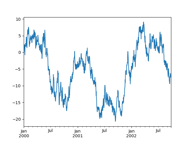
In [69]: ts = pd.Series(np.random.randn(1000),
   ....:                index=pd.date_range('1/1/2000', periods=1000))
   ....:

In [70]: ts = ts.cumsum()

In [71]: ts.plot()
Out[71]: <AxesSubplot: >
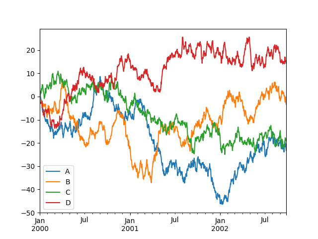
On a DataFrame, the plot() method is a convenience to plot all
of the columns with labels:
In [72]: df = pd.DataFrame(np.random.randn(1000, 4), index=ts.index,
   ....:                   columns=['A', 'B', 'C', 'D'])
   ....:

In [73]: df = df.cumsum()

In [74]: plt.figure()
Out[74]: <Figure size 640x480 with 0 Axes>

In [75]: df.plot()
Out[75]: <AxesSubplot: >

In [76]: plt.legend(loc='best')
Out[76]: <matplotlib.legend.Legend at 0x7f2005c1f280>
Getting data in/out#
CSV#
Writing to a csv file.
In [77]: df.to_csv('foo.csv')
Out[77]:
Empty DataFrame
Columns: []
Index: []
Reading from a csv file.
In [78]: pd.read_csv('foo.csv')
Out[78]:
     Unnamed: 0          A         B          C          D
0    2000-01-01  -0.709526  0.653838   0.527212  -2.549783
1    2000-01-02   0.665302  0.070092   0.058578  -2.683909
2    2000-01-03   0.073105 -2.063803  -0.095255  -2.918564
3    2000-01-04   0.016668 -1.389536   1.293680  -2.902580
4    2000-01-05  -1.015901 -2.870125   2.450304  -2.458862
..          ...        ...       ...        ...        ...
995  2002-09-22 -19.682572 -2.467442 -17.726526  15.666027
996  2002-09-23 -21.591296 -1.266325 -18.573105  15.012763
997  2002-09-24 -20.442837 -0.177719 -19.124194  15.582987
998  2002-09-25 -22.149444 -1.128729 -18.201630  15.076183
999  2002-09-26 -23.198270 -3.307830 -18.243414  14.363178

[1000 rows x 5 columns]